
Bigmart Sales Prediction Analysis using Python | Regression | Machine Learning Project Tutorial
- Hackers Realm
- Mar 28, 2022
- 7 min read
Updated: Jun 5, 2023
Unlock the secrets of Bigmart sales prediction with Python! This project tutorial delves into regression and machine learning, enabling you to forecast sales. Explore data preprocessing, feature engineering, and model evaluation. Gain practical experience with regression algorithms like linear regression, decision trees, and random forests. Supercharge your Python programming, data analysis, and machine learning skills. Dominate the art of Bigmart sales prediction! #BigmartSalesPrediction #Python #Regression #MachineLearning #DataAnalysis

In this project tutorial, we will analyze and predict the sales of Bigmart. Furthermore, we will operate one-hot encoding to improve the accuracy of our prediction models.
You can watch the video-based tutorial with step by step explanation down below
Dataset Information
The data scientists at BigMart have collected 2013 sales data for 1559 products across 10 stores in different cities. Also, certain attributes of each product and store have been defined. The aim is to build a predictive model and find out the sales of each product at a particular store.
Using this model, BigMart will try to understand the properties of products and stores which play a key role in increasing sales.

Download the Dataset here
Import modules
Let us import all the basic modules we will be needing for this project.
import pandas as pd
import numpy as np
import seaborn as sns
import matplotlib.pyplot as plt
import warnings
%matplotlib inline
warnings.filterwarnings('ignore')
pandas - used to perform data manipulation and analysis
numpy - used to perform a wide variety of mathematical operations on arrays
matplotlib - used for data visualization and graphical plotting
seaborn - built on top of matplotlib with similar functionalities
%matplotlib - to enable the inline plotting.
warnings - to manipulate warnings details
filterwarnings('ignore') is to ignore the warnings thrown by the modules (gives clean results)
Loading the dataset
df = pd.read_csv('Train.csv')
df.head()
# statistical info
df.describe()
We will fill the missing values using the range values (mean, minimum and maximum values).
# datatype of attributes
df.info()
We have categorical as well as numerical attributes which we will process separately.
# check unique values in dataset
df.apply(lambda x: len(x.unique()))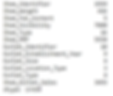
Attributes containing many unique values are of numerical type. The remaining attributes are of categorical type.
Preprocessing the dataset
Let us check for NULL values in the dataset.
# check for null values
df.isnull().sum()
We observe two attributes with many missing values (Item_Weight and Outlet_Size).
# check for categorical attributes
cat_col = []
for x in df.dtypes.index:
    if df.dtypes[x] == 'object':
        cat_col.append(x)
cat_col
For loop gets the columns from the datasets. If the datatype of these columns is equal to the object, then it will be added to the categorical attributes.
Above shown are the categorical columns of the dataset.
We can eliminate a few columns like 'Item_Identifier' and 'Outlet_Identifier'.
Let us remove unnecessary columns.
cat_col.remove('Item_Identifier')
cat_col.remove('Outlet_Identifier')
cat_col
The remaining are the necessary columns for this project.
Let's print the categorical columns.
# print the categorical columns
for col in cat_col:
    print(col)
    print(df[col].value_counts())
    print()

value_counts() - displays the number of counts for that particular value.
We will combine the repeated attributes which represents the same information.
We can also combine the attributes which contain low values. This practice will boost our prediction.
Let us now fill in the missing values.
# fill the missing values
item_weight_mean = df.pivot_table(values = "Item_Weight", index = 'Item_Identifier')
item_weight_mean
We have calculated the mean based on the 'Item_Identifier'.
pivot_table() is used to create a categorical column and fill the missing values based on those categories.
As a result, we have the average weight of each row of Item_Identifer.
Let's check for the missing values of Item_Weight.
miss_bool = df['Item_Weight'].isnull()
miss_bool
Rows will be represented as (True when having missing values) or (False when there are no missing values.)
In the case of True, we will fill the missing values for that row.
Let's fill in the missing values of Item_weight.
for i, item in enumerate(df['Item_Identifier']):
    if miss_bool[i]:
        if item in item_weight_mean:
            df['Item_Weight'][i] = item_weight_mean.loc[item]['Item_Weight']
        else:
df['Item_Weight'][i] = np.mean(df['Item_Weight'])df['Item_Weight'].isnull().sum()0
We have iterated in terms of Item_Identifier.
This if-else condition will get the average weight of that particular item and assigned it to that particular row.
As a result, the missing values has been filled with the average weight of that item.
Let's check for the missing values of Outler_Type.
outlet_size_mode = df.pivot_table(values='Outlet_Size', columns='Outlet_Type', aggfunc=(lambda x: x.mode()[0]))
outlet_size_mode
We use the aggregation function from the pivot table.
Since the Outlet_Type is a categorical attribute we will use Mode. In the case of numerical attributes, we have to use mean or median.
Let's fill in the missing values for Outlet_Size.
miss_bool = df['Outlet_Size'].isnull()
df.loc[miss_bool, 'Outlet_Size'] = df.loc[miss_bool, 'Outlet_Type'].apply(lambda x: outlet_size_mode[x])df['Outlet_Size'].isnull().sum()0
In the subscript of location operation, we have set a condition for filling the missing values for 'Outlet_Size'.
As a result, it will fill the missing values.
Similarly, we can check for Item_Visibility.
sum(df['Item_Visibility']==0)526
We have some missing values for this attribute.
Let's fill in the missing values.
# replace zeros with mean
df.loc[:, 'Item_Visibility'].replace([0], [df['Item_Visibility'].mean()], inplace=True)sum(df['Item_Visibility']==0)0
inplace=True, will keep the changes in the dataframe.
All the missing values are now filled.
Let us combine the repeated Values of the categorical column.
# combine item fat contentdf['Item_Fat_Content'] = df['Item_Fat_Content'].replace({'LF':'Low Fat', 'reg':'Regular', 'low fat':'Low Fat'})
df['Item_Fat_Content'].value_counts()
It will combine the values into two separate categories (Low Fat and Regular).
Creation of New Attributes
We can create new attributes 'New_Item_Type' using existing attributes 'item_Identifier'.
df['New_Item_Type'] = df['Item_Identifier'].apply(lambda x: x[:2])
df['New_Item_Type']
After creating a new attribute, let's fill in some meaningful value in it.
df['New_Item_Type'] = df['New_Item_Type'].map({'FD':'Food', 'NC':'Non-Consumable', 'DR':'Drinks'})
df['New_Item_Type'].value_counts()
Map or Replace is used to change the values.
We have three categories of (Food, Non-Consumables and Drinks).
We will use this 'Non_Consumable' category to represent the 'Fat_Content' which are 'Non-Edible'.
df.loc[df['New_Item_Type']=='Non-Consumable', 'Item_Fat_Content'] = 'Non-Edible'
df['Item_Fat_Content'].value_counts()
This will create another category for 'Item_Fat_Content'.
Let us create a new attribute to show small values for the establishment year.
# create small values for establishment year
df['Outlet_Years'] = 2013 - df['Outlet_Establishment_Year']
df['Outlet_Years']
It will return the difference between 2013 (when the dataset was collected) and the 'Outlet_Establishment_Year', and store it into the new attribute "Outlet_Years'.
Since the values are smaller than the previous, it will improve our model performance.
Let's print the dataframe.
df.head()
Exploratory Data Analysis
Let us explore the numerical columns.
sns.distplot(df['Item_Weight'])
We observe higher mean values.
And many items don't have enough data, thus showing zero.
sns.distplot(df['Item_Visibility'])
We have filled zero values with the mean, and it shows a left-skewed curve.
All the values are small. Hence, we don't have to worry about normalizing the data.
sns.distplot(df['Item_MRP'])
This graph shows four peak values.
Using this attribute we can also create other categories depending on the cost.
sns.distplot(df['Item_Outlet_Sales'])
The values are high and the curve is left-skewed.
We will normalize this using log transformation.
Log transformation helps to make the highly skewed distribution less skewed.
# log transformation
df['Item_Outlet_Sales'] = np.log(1+df['Item_Outlet_Sales'])sns.distplot(df['Item_Outlet_Sales'])
After using log transformation, the curve is normalized.
Let us explore the categorical columns.
sns.countplot(df["Item_Fat_Content"])
We observe that most items are low-fat content.
# plt.figure(figsize=(15,5))
l = list(df['Item_Type'].unique())
chart = sns.countplot(df["Item_Type"])
chart.set_xticklabels(labels=l, rotation=90)

plt.figure() is to increase the figure size.
chart.set_xticklabels() is to display the labels in a vertical manner as shown in the graph.
sns.countplot(df['Outlet_Establishment_Year'])
Most outlets are established in an equal distribution.
sns.countplot(df['Outlet_Size'])
sns.countplot(df['Outlet_Location_Type'])
sns.countplot(df['Outlet_Type'])
You can also combine the low values into one category.
Correlation Matrix
A correlation matrix is a table showing correlation coefficients between variables. Each cell in the table shows the correlation between two variables. The value is in the range of -1 to 1. If two variables have a high correlation, we can neglect one variable from those two.
corr = df.corr()
sns.heatmap(corr, annot=True, cmap='coolwarm')
Since we have derived 'Outlet_Years' from 'Oulet_Establishment_Year', we can observe a highly negative correction between these two.
And a positive correlation is between 'Item_MRP' and 'Item_Outlet_Sales'.
Let's check the values of the dataset.
df.head()
Label Encoding
Label encoding is to convert the categorical column into the numerical column.
from sklearn.preprocessing import LabelEncoder
le = LabelEncoder()
df['Outlet'] = le.fit_transform(df['Outlet_Identifier'])
cat_col = ['Item_Fat_Content', 'Item_Type', 'Outlet_Size', 'Outlet_Location_Type', 'Outlet_Type', 'New_Item_Type']
for col in cat_col:
    df[col] = le.fit_transform(df[col])
We access each column from the 'cat col' list. For the corresponding column, the le.fit_transform() function will convert the values into numerical then store them into the corresponding column.
One Hot Encoding
We can also use one hot encoding for the categorical columns.
df = pd.get_dummies(df, columns=['Item_Fat_Content', 'Outlet_Size', 'Outlet_Location_Type', 'Outlet_Type', 'New_Item_Type'])
df.head()
It will create a new column for each category. Hence, it will add the corresponding category instead of numerical values.
If the corresponding location type is present it will show as '1', or else it will show '0'.
We have around 26 features, which may increase the training time.
Splitting the data for Training and Testing
Let us drop some columns before training our model.
X = df.drop(columns=['Outlet_Establishment_Year', 'Item_Identifier', 'Outlet_Identifier', 'Item_Outlet_Sales'])
y = df['Item_Outlet_Sales']
Model Training
Now the preprocessing has been done, let's perform the model training and testing.
Note: Don't train & test with full data like below; split data for training and testing. For this project, consider the cross validation score for comparing the model performance
from sklearn.model_selection import cross_val_score
from sklearn.metrics import mean_squared_error
def train(model, X, y):
    # train the model
    model.fit(X, y)

    # predict the training set
    pred = model.predict(X)

    # perform cross-validation
    cv_score = cross_val_score(model, X, y, scoring='neg_mean_squared_error', cv=5)
    cv_score = np.abs(np.mean(cv_score))

    print("Model Report")
    print("MSE:",mean_squared_error(y,pred))
    print("CV Score:", cv_score)
X contains input attributes and y contains the output attribute.
We use 'cross val score()' for better validation of the model.
Here, cv=5 means that the cross-validation will split the data into 5 parts.
np.abs() will convert the negative score to positive and np.mean() will give the average value of 5 scores.
Linear Regression:
from sklearn.linear_model import LinearRegression, Ridge, Lasso
model = LinearRegression(normalize=True)
train(model, X, y)
coef = pd.Series(model.coef_, X.columns).sort_values()
coef.plot(kind='bar', title="Model Coefficients")
Model report: MSE = 0.288 CV Score = 0.289

The positive values are attributes with positive coefficients and negative values are attributes with negative coefficients.
There are minor values between positive and negative coefficients. This indicates that the centre attributes do not provide significant information.
Ridge:
model = Ridge(normalize=True)
train(model, X, y)
coef = pd.Series(model.coef_, X.columns).sort_values()
coef.plot(kind='bar', title="Model Coefficients")
Model report: MSE = 0.142 CV Score = 0.429

Lasso:
model = Lasso()
train(model, X, y)
coef = pd.Series(model.coef_, X.columns).sort_values()
coef.plot(kind='bar', title="Model Coefficients")
Model report: MSE = 0.762 CV Score = .763

Both the MSE and CV score is increasing.
Let's try some advanced models
Decision Tree:
from sklearn.tree import DecisionTreeRegressor
model = DecisionTreeRegressor()
train(model, X, y)
coef = pd.Series(model.feature_importances_, X.columns).sort_values(ascending=False)
coef.plot(kind='bar', title="Feature Importance")
Model report: MSE = 2.7767015e-34 CV Score = 0.567651

Random Forest:
from sklearn.ensemble import RandomForestRegressor
model = RandomForestRegressor()
train(model, X, y)
coef = pd.Series(model.feature_importances_, X.columns).sort_values(ascending=False)
coef.plot(kind='bar', title="Feature Importance")
Model report: MSE = 0.04191 CV Score = 0.30664

Extra Trees:
from sklearn.ensemble import ExtraTreesRegressor
model = ExtraTreesRegressor()
train(model, X, y)
coef = pd.Series(model.feature_importances_, X.columns).sort_values(ascending=False)
coef.plot(kind='bar', title="Feature Importance")
Model report: MSE = 1.0398099e-28 CV Score = 0.3295

The MSE has decreased, but the CV score is greater than the random forest.
Final Thoughts
Out of the 6 models, linear regression is the top performer with the least cv score.
You can also use hyperparameter tuning to improve the model performance.
You can further try other models like XGBoost, CatBoost etc.
In this project tutorial, we have explored the Bigmart Sales dataset. We learned the uses of one hot encoding in the dataset. We also compared different models to train the data starting from basic to advanced models.
Get the project notebook from here
Thanks for reading the article!!!
Check out more project videos from the YouTube channel Hackers Realm