
Handle Imbalanced classes in Dataset | Machine Learning | Python
- Hackers Realm
- Jul 17, 2023
- 8 min read

Updated: Aug 20, 2023
Imbalanced classes refer to a situation where the distribution of classes in a dataset is highly skewed, with one or more classes being significantly underrepresented compared to the others. Imbalanced classes can pose challenges in machine learning tasks because models trained on such data tend to have a bias towards the majority class. This bias can lead to poor predictive performance for the minority class, as the model may struggle to learn from the limited number of minority class examples.
Handling imbalanced classes in a dataset is an important aspect of machine learning, as it ensures that the model does not become biased towards the majority class and can effectively learn from the minority class as well. The strategies including resampling techniques (undersampling, oversampling, or a combination), class weighting, algorithmic techniques, ensemble methods, anomaly detection, data augmentation, and collecting more data. These techniques aim to rebalance the class distribution, provide more weight or focus to the minority class, or generate additional samples to improve the model's ability to learn from the minority class.
You can watch the video-based tutorial with step by step explanation down below.
Let us first see an example of Imbalanced class. For that we are using credit card data.
Import Module
from collections import CounterThe Counter class from the collections module is a useful tool for counting the frequency of elements in a list or any iterable.
Load the dataset
We will read the credit card data.
df = pd.read_csv('data/creditcard.csv')
df.head()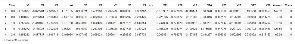
The code snippet reads a CSV file named 'creditcard.csv' into a Pandas DataFrame object named 'df' and then displaying the first few rows of the DataFrame using the head() function.
Next let us get the input and output split.
X = df.drop(columns=['Class'], axis=1)
y = df['Class']
X is assigned the DataFrame df with the 'Class' column dropped using the drop() function. The drop() function is used to remove specified columns from the DataFrame, and the columns parameter accepts a list of column names to be dropped. The axis=1 argument specifies that the columns should be dropped.
y is assigned the 'Class' column from the DataFrame df, which represents the target variable.
Next let us visualize the data
sns.countplot(y)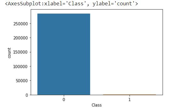
The countplot function from Seaborn is used to create a bar plot of the counts of each class in the target variable y. Calling plt.show() will display the plot.
This count plot provides a visual representation of the class distribution in y. Each bar represents the count of occurrences for each class. It can help you quickly identify any class imbalance in the data and assess the need for addressing it using the techniques mentioned earlier.
Next let us obtain the count of each class in the target variable y.
Counter(y)Counter({0: 284315, 1: 492})
The Counter function takes an iterable as input and returns a dictionary-like object with elements as keys and their frequencies as values. In this case, y represents the target variable, and calling Counter(y) will provide a count of occurrences for each class.
We can see that class 0 has 284315 samples and class 1 has only 492 samples. So this dataset is imbalanced. We have to have uniform distribution for better performance of the model . So to achieve uniform distribution we apply two techniques that is Over sampling and Under sampling.
Over Sampling Techniques
Oversampling techniques are used to address class imbalance by increasing the representation of the minority class in a dataset. These techniques create synthetic samples of the minority class to balance the class distribution.
First let us use Random Oversampling technique.
RandomOverSampler
Randomly duplicating samples from the minority class to increase its representation. This technique may lead to overfitting if the same samples are repeated too frequently.
Let us see the use of RandomOverSampler class from the imblearn.over_sampling module to perform random oversampling on the dataset.
from imblearn.over_sampling import RandomOverSampler
oversampler = RandomOverSampler(sampling_strategy='minority')
X_over, y_over = oversampler.fit_resample(X, y)
Counter(y_over)
Counter({0: 284315, 1: 284315})
RandomOverSampler is initialized with the parameter sampling_strategy='minority', which specifies that the oversampling should be applied to the minority class in order to balance the class distribution.
The fit_resample() method is then called on the oversampler object, passing X (features) and y (target) as arguments. This method applies the oversampling technique to the data and returns the oversampled versions of X and y, stored in X_over and y_over, respectively.
Finally, the Counter function is used to count the occurrences of each class in the oversampled target variable y_over.
We can see that class 0 has samples and class 1 also has 284315 samples. It has oversampled all the data in class 1. Here it has just randomly replicated the existing 492 samples in class 1 into 284315 samples. But this will overfit the data because of duplication so this cannot be considered as a best approach.
If you don't want to oversample to exactly 284315 samples and If you want to oversample the minority class to have a specific ratio or proportion relative to the majority class, you can use the RandomOverSampler with the sampling_strategy parameter set to a float value representing the desired ratio.
Next let us use the RandomOverSampler with the sampling_strategy parameter set to a float value representing the desired ratio.
oversampler = RandomOverSampler(sampling_strategy=0.3)
X_over, y_over = oversampler.fit_resample(X, y)
Counter(y_over)
Counter({0: 284315, 1: 85294})
sampling_strategy=0.3 indicates that you want to oversample the minority class to have a ratio of 0.3 (or 30%) relative to the majority class
By calling fit_resample() on the oversampler object with X and y as input, you obtain the oversampled versions in X_over and y_over, respectively.
Finally, the Counter function is used to count the occurrences of each class in the oversampled target variable y_over.
Now we can see that we got 85294 samples for class 1 . This is better compared to 284315 duplicates. However it is not the best approach as it will duplicate the data.
To overcome this we have another technique known as SMOTE. Let us see how this technique works.
SMOTE (Synthetic Minority Over-sampling Technique)
SMOTE generates synthetic samples by interpolating between minority class samples. It selects a minority class sample, finds its nearest neighbors, and creates new samples along the line segments connecting the sample with its neighbors. This technique helps to introduce more diverse synthetic samples.
Let us see the usage of SMOTE with a specific sampling strategy, where the minority class is oversampled to achieve a desired ratio compared to the majority class.
from imblearn.over_sampling import SMOTE
oversampler = SMOTE(sampling_strategy=0.4)
X_over, y_over = oversampler.fit_resample(X, y)
Counter(y_over)
Counter({0: 284315, 1: 113726})
sampling_strategy=0.4 specifies that you want to oversample the minority class to have a ratio of 0.4 (or 40%) relative to the majority class.
By calling fit_resample() on the oversampler object with X and y as input, you obtain the oversampled versions in X_over and y_over, respectively.
Finally, the Counter function is used to count the occurrences of each class in the oversampled target variable y_over.
We can see that class 0 has 284315 samples and class 1 also has 113726 samples. It has oversampled the data in class 1 by creating new samples which is better than RandomOverSampler technique.
Next let us visualize the data.
sns.countplot(y_over)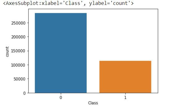
The countplot function from Seaborn is used to create a bar plot of the counts of each class in the oversampled target variable y_over. Calling plt.show() will display the plot.
This count plot provides a visual representation of the class distribution after oversampling. Each bar represents the count of occurrences for each class. It can help you assess whether the oversampling technique successfully balanced the classes or achieved the desired ratio.
Under Sampling Technique
Under sampling techniques are used to address class imbalance by reducing the number of samples from the majority class to match the number of samples in the minority class.
For Under Sampling we can randomly remove some of the existing data so we just go for Random Under Sampling technique
RandomUnderSampler
Randomly removing samples from the majority class to reduce its representation. This technique may discard potentially valuable information if the removed samples contain important patterns.
Let us see the use of the RandomUnderSampler class from the imblearn.under_sampling module to perform random under sampling on the dataset.
from imblearn.under_sampling import RandomUnderSampler
undersampler = RandomUnderSampler(sampling_strategy='majority')
X_under, y_under = undersampler.fit_resample(X, y)
Counter(y_under)
Counter({0: 492, 1: 492})
RandomUnderSampler is initialized with the parameter sampling_strategy='majority', which specifies that the under sampling should be applied to the majority class to balance the class distribution.
The fit_resample() method is then called on the undersampler object, passing X (features) and y (target) as arguments. This method applies the under sampling technique to the data and returns the under-sampled versions of X and y, stored in X_under and y_under, respectively.
Finally, the Counter function is used to count the occurrences of each class in the under-sampled target variable y_under.
We can see that now class 0 samples has been reduced from 284315 samples to 492 samples same as class 1. Here we have seen that majority of samples has been removed .
We can also increase the samples of class 0 to a certain percentage.
undersampler = RandomUnderSampler(sampling_strategy=0.2)
X_under, y_under = undersampler.fit_resample(X, y)
Counter(y_under)
Counter({0: 2460, 1: 492})
sampling_strategy=0.2 indicates that you want to under-sample the majority class to have a ratio of 0.2 (or 20%) relative to the minority class.
By calling fit_resample() on the undersampler object with X (features) and y (target) as input, you obtain the under-sampled versions in X_under and y_under, respectively.
Finally, the Counter function is used to count the occurrences of each class in the under-sampled target variable y_under.
We can see that class 0 samples has been increased to 20% of class 1 samples.
Next let us visualize the data
sns.countplot(y_under)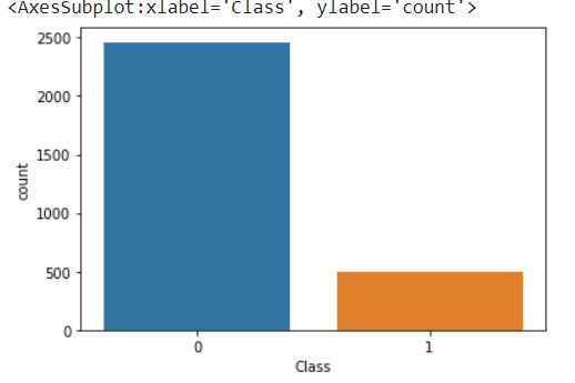
Combine Oversampling and Undersampling
Let us create a pipeline to perform oversampling and undersampling.
from imblearn.pipeline import Pipeline
over = SMOTE(sampling_strategy=0.1)
under = RandomUnderSampler(sampling_strategy=0.5)
pipeline = Pipeline([('o', over), ('u', under)])
X_resample, y_resample = pipeline.fit_resample(X, y)
A pipeline is created using the Pipeline class. The pipeline consists of two steps, denoted by a list of tuples.
The first step, named 'o', represents the oversampling step, which uses SMOTE with a sampling strategy of 0.1 (or 10%).
The second step, named 'u', represents the undersampling step, which uses RandomUnderSampler with a sampling strategy of 0.5 (or 50%).
By calling fit_resample() on the pipeline with X (features) and y (target) as input, you obtain the resampled versions in X_resample and y_resample, respectively.
The pipeline applies the oversampling and undersampling techniques in sequence, ensuring that both steps are performed in a consistent manner.
You can then use X_resample and y_resample for further analysis or model training with a more balanced class distribution achieved through the combined oversampling and undersampling techniques.
Next let us visualize the data. First we will plot the original data.
sns.countplot(y)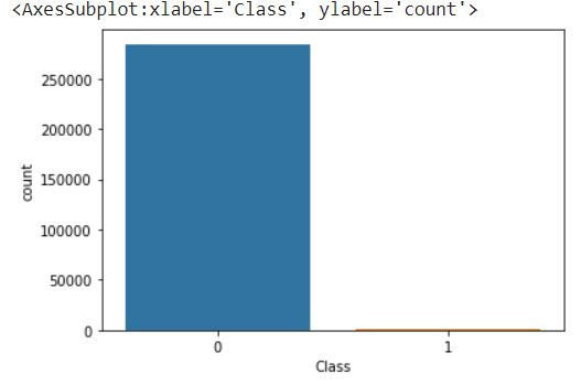
Let us plot the data after resampling it.
sns.countplot(y_resample)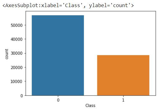
We can see the difference that for class 0 from 284315 samples it has reduced to around 60000 samples and for class 1 from 492 samples it has increased to around 28000 samples.
Final Thoughts
Gain a thorough understanding of the problem domain, the class distribution, and the potential impact of class imbalance on model performance and evaluation.
Perform exploratory data analysis to understand the characteristics of each class, identify potential challenges, and detect any patterns or anomalies.
Select evaluation metrics that are robust to imbalanced classes, such as precision, recall, F1-score, area under the precision-recall curve (AUPRC), or balanced accuracy.
Cleanse the data, handle missing values, and apply appropriate feature engineering techniques to enhance the representation of both the majority and minority classes.
Employ resampling techniques, such as oversampling or undersampling, to rebalance the class distribution. Choose the appropriate technique based on the dataset characteristics and consider using combinations or hybrid approaches.
Use proper cross-validation techniques to validate the model's performance, ensuring that it generalizes well to unseen data. Monitor performance on both majority and minority classes to ensure balanced performance.
Seek guidance from domain experts to better understand the impact of misclassification for different classes and incorporate domain-specific knowledge into model development.
Handling imbalanced classes often involves an iterative process of trying different techniques, evaluating their impact, and refining the approach based on feedback and insights gained from the data.
In this article we have explored how we can handle imbalanced classes using Oversampling and Under Sampling techniques. In future we can explore other methods that can also be used to handle the imbalanced classes in dataset.
Get the project notebook from here
Thanks for reading the article!!!
Check out more project videos from the YouTube channel Hackers Realm


Comments