
How to Handle Large Dataset (Pandas CSV) | Python
- Hackers Realm
- Nov 11, 2023
- 9 min read

Updated: Apr 27, 2024
Conquer large datasets with Pandas in Python! This tutorial unveils strategies for efficient CSV handling, optimizing memory usage. Whether you're a novice or an experienced data wrangler, learn step-by-step techniques to streamline your workflow and enhance data processing speed. Dive into memory management, chunking, and parallel processing to master handling large datasets with ease. Join us on this illuminating journey to empower your Python skills and efficiently manage vast amounts of data. #LargeDataset #Pandas #CSVHandling #Python #DataProcessing

In this tutorial, we will explore the challenges and strategies associated with the handling of large datasets. We will delve into various aspects of data management, storage, processing, and analysis, equipping you with the skills and knowledge needed to navigate the complexities of working with big data.
You can watch the video-based tutorial with a step-by-step explanation down below.
Load the dataset
First we will load the dataset.
df = pd.read_csv('data/1000000 Sales Records.csv')
df.head()
pd.read_csv('data/1000000 Sales Records.csv') is a Pandas function that reads data from a CSV (Comma-Separated Values) file. It takes the path to the CSV file as an argument and returns a Pandas DataFrame, which is a two-dimensional, tabular data structure for working with data.
df.head() is a method applied to the DataFrame df. It is used to display the first few rows of the DataFrame to get a quick overview of the data.
Next we will see detailed information about the DataFrame df.
df.info(verbose=False, memory_usage='deep')<class 'pandas.core.frame.DataFrame'>
RangeIndex: 1000000 entries, 0 to 999999
Columns: 14 entries, Region to Total Profit
dtypes: float64(5), int64(2), object(7)
memory usage: 489.9 MB
df.info(): This is a Pandas DataFrame method that provides essential information about the DataFrame, such as the number of non-null values, data types, and memory usage. By default, it's quite verbose and displays all these details.
verbose=False: By setting verbose to False, you're suppressing some of the more detailed information that would normally be displayed when using df.info(). This can make the output less extensive and easier to read, especially for large DataFrames.
memory_usage='deep': Setting memory_usage to 'deep' makes df.info() calculate the memory usage of the DataFrame more accurately. It takes into account the memory used by the actual data and any additional memory overhead that might be present due to the internal data structures in Pandas. This is useful when you want a precise measurement of memory consumption.
Let's analyze the output -> <class 'pandas.core.frame.DataFrame'> - This line tells you that the variable df is of the class 'pandas.core.frame.DataFrame'. -> RangeIndex: 1000000 entries, 0 to 999999 - This line provides information about the index of the DataFrame. It's a "RangeIndex" with 1,000,000 entries, indicating that your DataFrame has 1,000,000 rows. The index is based on integers, ranging from 0 to 999,999. -> Columns: 14 entries, Region to Total Profit -This line lists the names of the columns in the DataFrame. -> dtypes: float64(5), int64(2), object(7) - This line provides information about the data types of the columns. -> memory usage: 489.9 MB - This line shows the estimated memory usage of the DataFrame. In this case, the memory usage is approximately 489.9 megabytes (MB).
We have analyzed the large dataset that we have loaded and observed that the memory usage is high. Now let us see some strategies for working efficiently with large datasets.
nrows
When working with very large datasets, it might not be practical to load the entire dataset into memory, as it can lead to high memory consumption. By using nrows, you can read only a subset of the data, which can be useful for initial data exploration and sampling without overloading your system's memory.
We will first load the dataset using nrows.
df = pd.read_csv('data/1000000 Sales Records.csv', nrows=1000)
df.info(verbose=False, memory_usage='deep')
<class 'pandas.core.frame.DataFrame'>
RangeIndex: 1000 entries, 0 to 999
Columns: 14 entries, Region to Total Profit
dtypes: float64(5), int64(2), object(7)
memory usage: 502.1 KB
Lets analyze the output : -> memory usage: 502.1 KB - This line shows the estimated memory usage of the DataFrame, which is approximately 502.1 kilobytes (KB).
We can see that the memory usage has drastically decreased when we loaded only 1000 rows.
Use Required Columns
Using only the required columns, or "column pruning," is a common technique to help in handling large datasets more efficiently
First we will extract the column names from dataframe.
cols = df.columns.values
cols
array(['Region', 'Country', 'Item Type', 'Sales Channel',
'Order Priority', 'Order Date', 'Order ID', 'Ship Date',
'Units Sold', 'Unit Price', 'Unit Cost', 'Total Revenue',
'Total Cost', 'Total Profit'], dtype=object)
df.columns: This is an attribute of a Pandas DataFrame that returns the column labels (names) of the DataFrame.
values: This is used to extract the values from the attribute, converting them into a NumPy array.
After executing this code, the variable cols will contain an array of the column names from the DataFrame df.
Next let us define the list of required columns.
req_cols = ['Region', 'Country', 'Item Type', 'Sales Channel',
       'Order Priority',
       'Units Sold', 'Unit Price', 'Unit Cost', 'Total Revenue',
       'Total Cost', 'Total Profit']
We created a list of required columns named req_cols. This list contains the names of the columns we want to retain from our DataFrame.
Next let us load the dataset with only required columns.
df = pd.read_csv('data/1000000 Sales Records.csv', usecols=req_cols)
df.head()
The code snippet reads a CSV file named '1000000 Sales Records.csv' and uses the usecols parameter to specify that you want to read only the columns listed in the req_cols list.
After reading the file, it displays the first few rows of the resulting DataFrame using df.head().
Next let us see a concise summary of the Pandas DataFrame df, focusing on memory usage and without displaying detailed column statistics.
df.info(verbose=False, memory_usage='deep')<class 'pandas.core.frame.DataFrame'>
RangeIndex: 1000000 entries, 0 to 999999
Columns: 11 entries, Region to Total Profit
dtypes: float64(5), int64(1), object(5)
memory usage: 356.5 MB
From the output we can conclude that the memory usage is reduced when compared to the memory consumed while loading the dataset with all the columns.
Convert Datatype of the Columns
Different data types require varying amounts of memory. By converting columns to more memory-efficient data types, you can significantly reduce the memory footprint of your dataset. Let us explore it with an example.
We can see that we have float64, int64, object datatypes. We will see min and max range of the columns and try to convert these datatypes.
df.describe()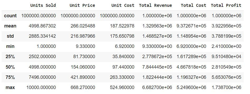
The df.describe() method in Pandas provides a summary of the statistics for numerical columns in a DataFrame. It calculates various statistical measures for each numeric column, such as count, mean, standard deviation, minimum, quartiles, and maximum. This summary can be helpful for gaining an initial understanding of your data's distribution and central tendencies.
Count: The number of non-null (non-missing) values in each column.
Mean: The average value of each column.
Std: The standard deviation, which measures the spread or variability of the data.
Min: The minimum (smallest) value in each column.
25%: The first quartile, which represents the 25th percentile or lower quartile.
50%: The median, which represents the 50th percentile or middle quartile.
75%: The third quartile, which represents the 75th percentile or upper quartile.
Max: The maximum (largest) value in each column.
Next we will convert the data types of the columns to more memory-efficient types.
for col in df.columns:
    if df[col].dtype == 'float64':
        df[col] = df[col].astype('float16')
    if df[col].dtype == 'int64':
        df[col] = df[col].astype('int16')
    if df[col].dtype == 'object':
        df[col] = df[col].astype('category')
The loop iterates through each column in the DataFrame using for col in df.columns.
Depending on the data type, it performs one of the following conversions. -> If the column has a data type of 'float64', it converts the column to the more memory-efficient data type 'float16'. -> If the column has a data type of 'int64', it converts the column to the more memory-efficient data type 'int16'. -> If the column has a data type of 'object', it converts the column to the data type 'category'. This can be useful for categorical data with a limited number of unique values and can save memory.
Smaller data types take up less memory, making your code more memory-efficient and potentially improving data processing speed.
Next let us see a concise summary of the Pandas DataFrame df, focusing on memory usage and without displaying detailed column statistics.
df.info(verbose=False, memory_usage='deep')<class 'pandas.core.frame.DataFrame'>
RangeIndex: 1000000 entries, 0 to 999999
Columns: 11 entries, Region to Total Profit
dtypes: category(5), float16(5), int16(1)
memory usage: 17.2 MB
From the output we can see that the memory usage is reduced from 356.5 MB to 17.2 MB.
The datatype conversion has drastically reduced the memory consumption.
Let us also see an example on how we can convert the datatypes while reading the dataset.
df = pd.read_csv('data/1000000 Sales Records.csv', usecols=req_cols, dtype={'Region': 'category', 'Units Sold': 'int16'})
df.info(verbose=False, memory_usage='deep')
<class 'pandas.core.frame.DataFrame'>
RangeIndex: 1000000 entries, 0 to 999999
Columns: 11 entries, Region to Total Profit
dtypes: category(1), float64(5), int16(1), object(4)
memory usage: 282.3 MB
usecols=req_cols specifies that you are reading only the columns listed in the req_cols list, which can significantly reduce memory usage if the original dataset had more columns.
dtype={'Region': 'category', 'Units Sold': 'int16'} specifies the data types for two specific columns. The 'Region' column is assigned the 'category' data type, which is memory-efficient for categorical data with a limited number of unique values. The 'Units Sold' column is assigned the 'int16' data type, which is a 16-bit integer, providing memory savings compared to the default 'int64' data type.
By using usecols to read only the necessary columns and specifying data types with dtype, we are efficiently managing memory and resources when working with a large dataset. This approach can make our data analysis more efficient and help prevent memory-related issues.
Here we have converted the datatypes of only two columns. With just converting the two columns datatype , the memory usage has reduced from 356.5 MB to 282.3 MB
Till now we have seen how we can load the dataset by using the memory efficiently. Now we will see how we can load the dataset 10 times faster.
Load Dataset Faster using chunks
First we will see the time taken to load the entire dataset
%%time
df = pd.read_csv('data/1000000 Sales Records.csv')
len(df)
Wall time: 2.1 s
1000000
%%time: This is a Jupyter Notebook magic command that is used to measure the execution time of the code in the cell. When we include %%time at the beginning of a cell, it will display timing information for the code that follows.
df = pd.read_csv('data/1000000 Sales Records.csv'): This line reads a CSV file named '1000000 Sales Records.csv' located in the 'data' directory using Pandas' pd.read_csv function.
len(df): This line calculates the length of the DataFrame 'df', which corresponds to the number of rows in the DataFrame. The len function is used to count the number of rows.
Wall time: This represents the actual elapsed time, which includes not only the time the CPU spends on the code but also any time the code spends waiting, for example, when reading from a file.
Here the wall time taken is 2.1 s to load 1000000 records.
Now we will load the data in chunks.
%%time
chunks = pd.read_csv('data/1000000 Sales Records.csv', iterator=True, chunksize=1000)
Wall time: 5.01 ms
iterator=True: By setting iterator to True, we are creating a CSV file iterator. This means that the file is not fully loaded into memory at once but rather read in smaller chunks as needed.
chunksize=1000: The chunksize parameter specifies the number of rows to be read at a time. In this case, it's set to 1000, which means that the file will be read in chunks of 1000 rows each.
This approach allows us to read the data in smaller, manageable chunks, which can be especially helpful when working with very large datasets. The use of an iterator and chunking helps reduce memory usage and allows us to process the data incrementally.
The time taken to load the dataset is reduced from 2.1 s to 5.01 ms .
Now let us verify if we have loaded all the records using chunks.
length = 0
for chunk in chunks:
    length += len(chunk)
length
1000000
The above code snippet is used to calculate the total number of rows in a CSV file '1000000 Sales Records.csv' by iteratively processing the file in chunks.
We can see that length of data loaded is 1000000 which is same as the data loaded at a time.
Final Thoughts
When dealing with very large datasets, consider taking random or systematic samples of the data for exploratory analysis. This allows you to gain insights without the need to process the entire dataset.
Use techniques like data chunking to read and process the data in smaller, manageable portions. This reduces memory usage and allows you to work with large datasets that can't fit entirely into memory.
Select only the columns that are relevant to your analysis. This reduces memory usage and speeds up data processing.
Choose appropriate data types for your columns to minimize memory usage. Smaller data types, like using int16 instead of int64 or category data types for categorical variables, can be very memory-efficient.
Utilize parallel processing and distributed computing frameworks (e.g., Dask, Apache Spark) to take advantage of multiple cores and distributed computing resources for faster data processing.
In this tutorial we have explored most of the strategies to handle large datasets. Further we can explore on other techniques which can help us in handling the large datasets more efficiently.
Get the project notebook from here
Thanks for reading the article!!!
Check out more project videos from the YouTube channel Hackers Realm


Comments