
Mastering Machine Learning with PySpark | Loan Prediction | Python
- Hackers Realm
- Jun 4, 2023
- 12 min read

The goal of this project tutorial is to demonstrate the use of PySpark and Machine Learning to predict loan approvals. The project will involve the following steps:
Data Collection: Collecting data related to loan approvals, including features such as income, credit score, loan amount, and loan status.
Data Preparation: Preprocessing and cleaning up the data to ensure it is ready for use in Machine Learning algorithms.
Feature Engineering: Selecting and engineering relevant features to improve the accuracy of the model.
Model Training: Using PySpark to train a Machine Learning model on the prepared data.
Model Evaluation: Testing the trained model on a validation set to evaluate its accuracy and adjust the parameters if necessary.
Loan Prediction: Using the trained model to predict whether a loan will be approved or not based on input features.

The project will require knowledge of PySpark, Machine Learning, and Python programming. The end result will be a Machine Learning model that can accurately predict loan approvals based on various features. This can be used by financial institutions or individuals to make more informed decisions regarding loans. Let us deep dive into the above mentioned steps
You can watch the video-based tutorial with step by step explanation down below.
Dataset Information
Dream Housing Finance company deals in all home loans. They have presence across all urban, semi urban and rural areas. Customer first apply for home loan after that company validates the customer eligibility for loan. Company wants to automate the loan eligibility process (real time) based on customer detail provided while filling online application form. These details are Gender, Marital Status, Education, Number of Dependents, Income, Loan Amount, Credit History and others. To automate this process, they have given a problem to identify the customers segments, those are eligible for loan amount so that they can specifically target these customers.
This is a standard supervised classification task. A classification problem where we have to predict whether a loan would be approved or not. Below is the dataset attributes with description
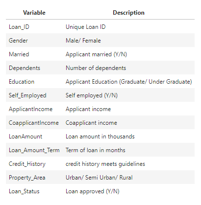
Download the Dataset here
Installing PySpark
Follow the below steps to install PySpark
Install Java
Install Apache spark with Hadoop
Set the environment variables
Next install pyspark using the command
!pip install pyspark
Import Modules
import pyspark
from pyspark.sql import SparkSession
import pyspark.sql.functions as F

import pandas as pd
import warnings
warnings.filterwarnings('ignore')
pyspark - It is a Python library and interface for Apache Spark, which is an open-source distributed computing system. PySpark allows you to write Spark applications using Python, leveraging the power and scalability of Spark for big data processing and analytics
pyspark.sql - provides a programming interface for working with structured data, such as structured data files, tables, and relational databases. It offers a high-level API for querying and manipulating structured data using SQL-like expressions and DataFrame operations
pyspark.sql.functions - provides a collection of built-in functions that can be used for data manipulation, transformation, and aggregation on DataFrame columns
pandas - used to perform data manipulation and analysis
warnings - to manipulate warnings details filterwarnings('ignore') is to ignore the warnings thrown by the modules (gives clean results)
Next we will initialize the spark session
# initialize the session
spark = SparkSession.builder.appName('loan_prediction').getOrCreate()
SparkSession is the entry point for any Spark functionality. It provides a way to interact with various Spark features, such as DataFrame and SQL operations, streaming, machine learning, and more
The builder pattern is used to create and configure the SparkSession. The builder method returns a Builder object that allows you to set various configuration options for the SparkSession
The appName method sets the name of the Spark application. In this case, it is set to "loan_prediction"
The getOrCreate method tries to reuse an existing SparkSession or creates a new one if it doesn't exist
Load the Dataset
Next we will load the dataset
df = spark.read.csv('Loan Prediction Dataset.csv', header=True, sep=',', inferSchema=True)
df.show(5)
spark.read.csv() function is used to read data from a CSV file and create a DataFrame
header=True option indicates that the first row of the CSV file contains the header or column names. By setting this option to True, the column names will be inferred from the header row
sep=',' option specifies the delimiter used in the CSV file. In this case, the delimiter is set to a comma (','), which is a common delimiter in CSV files
inferSchema=True option instructs Spark to automatically infer the data types for each column in the DataFrame based on the contents of the CSV file
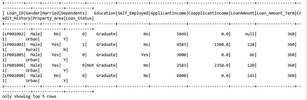
This is the first 5 rows of the DataFrame
Next let us see the schema of DataFrame
df.printSchema()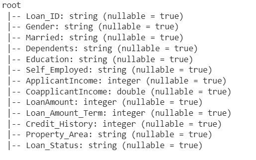
Next let us see the data types of columns
df.dtypes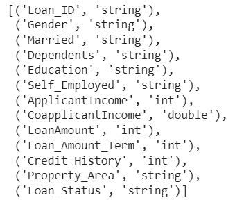
Next let us convert spark DataFrame to pandas DataFrame
# convert spark dataframe to pandas
pandas_df = df.toPandas()
pandas_df.head()
The toPandas() method is used to convert a PySpark DataFrame to a Pandas DataFrame. It collects the data from the distributed Spark DataFrame and brings it into a single machine's memory as a Pandas DataFrame
The resulting Pandas DataFrame pandas_df contains the same data as the original PySpark DataFrame df, but it is now in a Pandas format, allowing you to use Pandas-specific operations and libraries for further analysis and processing

Data Analysis
First let us display count based on loan status
# display count based on loan status
df.groupBy('Loan_Status').count().show()
df.groupBy() groups the DataFrame df by the 'Loan_Status' column. It creates a GroupedData object that allows you to perform aggregation operations on the grouped data
count() function is an aggregation function that calculates the number of non-null values in each group. In this case, it counts the occurrences of each unique value in the 'Loan_Status' column within each group
show() function is used to display the result of the aggregation operation
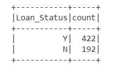
We can see that the count of status Y is 422 and status N is 192
Next let us perform grouping and aggregation operation on the DataFrame
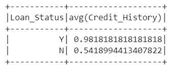
df.select("Credit_History", "Loan_Status").groupBy('Loan_Status').agg(F.avg('Credit_History')).show()The above code snippet selects the columns "Credit_History" and "Loan_Status" from the DataFrame, groups the data by the "Loan_Status" column, and then calculates the average of the "Credit_History" column for each group
Next we will perform grouping and counting operation on the DataFrame
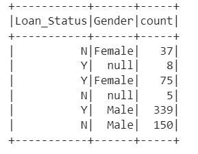
df.select('Gender', 'Loan_Status').groupBy('Loan_Status', 'Gender').count().show()It selects the columns 'Gender' and 'Loan_Status' from the DataFrame, groups the data by both 'Loan_Status' and 'Gender', and then counts the number of occurrences for each combination
Correlation Matrix
Next we will create a correlation matrix
columns = ['ApplicantIncome', 'CoapplicantIncome', 'LoanAmount', 'Loan_Amount_Term', 'Credit_History']
corr_df = pd.DataFrame()
for i in columns:
corr = []
for j in columns:
corr.append(round(df.stat.corr(i, j), 2))
corr_df = pd.concat([corr_df, pd.Series(corr)], axis=1)
corr_df.columns = columns
corr_df.insert(0, '', columns)
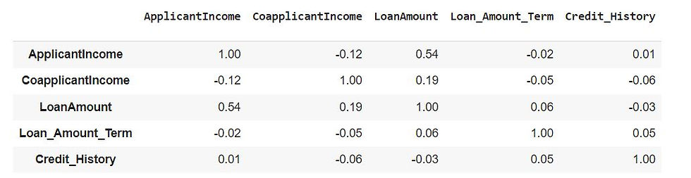
corr_df.set_index('')We will calculate the correlation matrix for the columns 'ApplicantIncome', 'CoapplicantIncome', 'LoanAmount', 'Loan_Amount_Term', 'Credit_History' in a DataFrame using the Pandas library
The correlation between each pair of columns is calculated using the corr() method on the corresponding columns in the DataFrame . The resulting correlation coefficients are rounded to two decimal places and stored in the corr_df DataFrame. The column names and index of corr_df are set
Perform SQL Operations
Next let us perform analysis using SQL operations
import pyspark.sql as sparksqlFirst we will import sparksql from pyspark
Next we will create a temporary view named "table" from the DataFrame df in Apache Spark. A temporary view allows you to query the DataFrame using SQL-like syntax
df.createOrReplaceTempView('table')Next we will display the top rows from the table
# display top rows from the table
spark.sql("select * from table limit 5").show()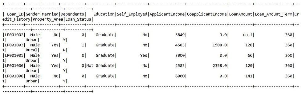
Next we will execute a sql query on the temporary view created
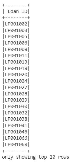
spark.sql('select Loan_ID from table where Credit_History=1').show()This will execute the SQL query on the "table" temporary view and display the result, which includes the Loan_ID values for rows where the Credit_History column equals 1
Data Preprocessing
First we will display the null values in the columns
# display null values
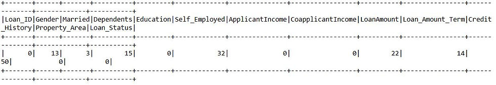
df.select([F.count(F.when(F.col(c).isNull(), c)).alias(c) for c in df.columns]).show()This uses the select function in Apache Spark to count the number of null values for each column in the DataFrame df and display the result
Next we will calculate the mean value of the column
# get mean value of column
mean = df.select(F.mean(df['LoanAmount'])).collect()[0][0]
mean
This calculates the mean value of the 'LoanAmount' column in the DataFrame df using the mean() function from the pyspark.sql.functions module
146.41216216216216
This is the mean value of the 'LoanAmount' column
Next we will fill the null values
# fill null value
df = df.na.fill(mean, ['LoanAmount'])
This fills the null values in the 'LoanAmount' column of the DataFrame df with the mean value
Next we will get mode value of a column
# get mode value of column
df.groupby('Gender').count().orderBy("count", ascending=False).first()[0]
'Male'
This performs a group by operation on the 'Gender' column of the DataFrame df, counts the number of occurrences for each gender, orders the result in descending order based on the count, and retrieves the first row. Finally, it returns the value in the first column of the first row, which corresponds to the gender with the highest count
Next we will fill the null values for all the columns
# fill null values for all the columns
numerical_cols = ['LoanAmount', 'Loan_Amount_Term']
categorical_cols = ['Gender', 'Married', 'Dependents', 'Self_Employed', 'Credit_History']
First we will create a list of numerical columns and categorical columns
Next let us first fill the null values for numerical columns
for col in numerical_cols:
    mean = df.select(F.mean(df[col])).collect()[0][0]
    df = df.na.fill(mean, [col])
This fills the null values in multiple numerical columns of the DataFrame df with their respective mean values. It iterates over each column name in the list numerical_cols, calculates the mean value for each column, and then fills the null values in that column with the corresponding mean value
Next let us fill the null values for categorical columns
for col in categorical_cols:
    mode = df.groupby(col).count().orderBy("count", ascending=False).first()[0]
    df = df.na.fill(mode, [col])
This fills the null values in multiple categorical columns of the DataFrame df with their respective mode values. It iterates over each column name in the list categorical_cols, calculates the mode value for each column, and then fills the null values in that column with the corresponding mode value
Now let us display the count of null values in the respective columns
# display null values
df.select([F.count(F.when(F.col(c).isNull(), c)).alias(c) for c in df.columns]).show()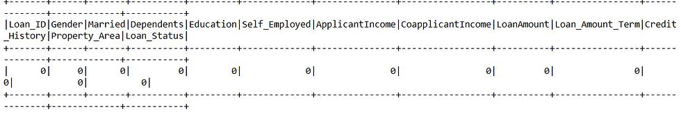
We can see that there is no null values in any columns
Next let us create new column
# create new feature column
df = df.withColumn('TotalIncome', F.col('ApplicantIncome') + F.col('CoapplicantIncome'))
df.show(2)
The withColumn() function is used to add a new column named 'TotalIncome' to the DataFrame df.
The new column is created by performing the addition operation F.col('ApplicantIncome') + F.col('CoapplicantIncome'), where F.col() is used to reference the corresponding columns
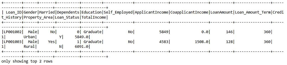
We can see that a new column TotalIncome is added with corresponding values
Let us see how we can find and replace the values
# how to find and replace values
df = df.withColumn('Loan_Status', F.when(df['Loan_Status']=='Y', 1).otherwise(0))
df.show(2)
The withColumn() function is used to add a new column named 'Loan_Status' to the DataFrame df.
The new column is created using the F.when() function, which checks the condition df['Loan_Status'] == 'Y'. If the condition is true, it assigns the value 1 to the 'Loan_Status' column; otherwise, it assigns the value 0 using the otherwise() function

We can see that Loan_Status column values are replaced with 1 and 0
Feature Engineering
Feature engineering is the process of transforming raw data into meaningful features that can improve the performance of a machine learning model. It involves creating new features or modifying existing features to capture patterns, relationships, or important information in the data that may be useful for the model's predictive task
First let us print the schema of the dataframe
df.printSchema()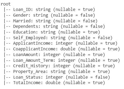
Next let us import required modules
from pyspark.ml.feature import VectorAssembler, OneHotEncoder, StringIndexer
from pyspark.ml import Pipeline
pyspark.ml.feature - provides various feature engineering techniques and transformations for machine learning tasks
pyspark.ml - provides a high-level API for building machine learning pipelines. It offers a set of tools and algorithms for various stages of the machine learning workflow, including feature extraction, transformation, model training, and evaluation
Next we will perform feature engineering workflow using pyspark.ml to handle categorical and numerical columns
categorical_columns = ['Gender', 'Married', 'Dependents', 'Education', 'Self_Employed', 'Property_Area', 'Credit_History']
numerical_columns = ['ApplicantIncome', 'CoapplicantIncome', 'LoanAmount', 'Loan_Amount_Term', 'TotalIncome']

# index the string columns
indexers = [StringIndexer(inputCol=col, outputCol="{0}_index".format(col)) for col in categorical_columns]

# encode the indexed values
encoders = [OneHotEncoder(dropLast=False, inputCol=indexer.getOutputCol(), outputCol="{0}_encoded".format(indexer.getOutputCol()))
           for indexer in indexers]

input_columns = [encoder.getOutputCol() for encoder in encoders] + numerical_columns

# vectorize the encoded values
assembler = VectorAssembler(inputCols=input_columns, outputCol="feature")
First we will create a list of categorical columns and a list of numerical columns that you want to process
The categorical columns are indexed using StringIndexer. Each categorical column is transformed into a numerical column with unique indices. A separate StringIndexer is created for each categorical column, and the output column names are suffixed with _index
Next, the indexed values are encoded using OneHotEncoder. Each indexed column is transformed into a binary vector representation, where each category is represented by a separate binary column. Again, a separate OneHotEncoder is created for each indexed column, and the output column names are suffixed with _encoded
The encoded values and the numerical columns are combined into a single list , which will serve as input for the subsequent steps.
Finally, the combined values are vectorized using VectorAssembler. The VectorAssembler takes the list of input columns and combines them into a single feature vector column named "features"
Next we will create a pipeline to transform data
# create the pipeline to transform the data
pipeline = Pipeline(stages = indexers + encoders + [assembler])
The Pipeline object is created with the specified stages, which include the indexers, encoders, and assembler steps. The stages are added to the pipeline using the + operator, and [assembler] is wrapped in a list to ensure it is passed as a single element
The Pipeline object allows you to chain together multiple stages into a single workflow, where each stage represents a transformation or modeling step. This enables you to streamline the feature engineering process and apply it consistently to different datasets
Next we will fit the pipeline into a dataframe
data_model = pipeline.fit(df)This fits the defined Pipeline object (pipeline) to the DataFrame df.
The fit() method applies each stage of the pipeline to the data sequentially, starting from the first stage and continuing through the subsequent stages
Next we will transform the data
transformed_df = data_model.transform(df)This applies the fitted PipelineModel (data_model) to the DataFrame df to perform the feature engineering transformations defined in the pipeline. The result is a new DataFrame transformed_df that contains the original columns from df along with the engineered features
The transform() method of a PipelineModel applies each transformation stage in the pipeline to the input DataFrame, starting from the first stage and sequentially passing the transformed output of each stage as input to the next stage
Next we will display the transformed dataframe
transformed_df.show(1)
Next let us get the input and output columns
# get input feature and output columns
transformed_df = transformed_df.select(['feature', 'Loan_Status'])
This selects the specified columns "feature" and "Loan_Status" from the DataFrame transformed_df and returns a new DataFrame that contains only those columns
Next let us split the train and test data
# split the data for train and test
train_data, test_data = transformed_df.randomSplit([0.8, 0.2], seed=42)
The randomSplit() method is called on the DataFrame transformed_df and takes two arguments
The first argument is a list [0.8, 0.2], which specifies the relative weights or proportions for splitting the data. In this case, it indicates that 80% of the data will be assigned to train_data, and 20% of the data will be assigned to test_data.
The second argument is the seed parameter, which sets a seed value for the random number generator. This ensures that the data is split in a consistent manner when the code is executed multiple times
Next let us display the train data
train_data.show(5)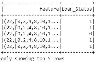
Model Training & Testing
First let us import the required modules
from pyspark.ml.classification import LogisticRegression, RandomForestClassifier
from pyspark.ml.evaluation import BinaryClassificationEvaluator
pyspark.ml.classification - provides classes and algorithms for performing classification tasks using machine learning. It includes various classification algorithms and evaluation metrics to train and evaluate classification models
pyspark.ml.evaluation - provides classes for evaluating the performance of machine learning models. It includes evaluation metrics for both binary and multiclass classification, as well as regression tasks
Next let us train logistic regression model
lr = LogisticRegression(featuresCol='feature', labelCol='Loan_Status')
lr_model = lr.fit(train_data)
The LogisticRegression class is used for binary classification tasks and implements logistic regression, which is a popular algorithm for modeling the probability of a binary outcome
The arguments featuresCol and labelCol specify the names of the columns in the DataFrame that contain the features and the target variable, respectively
After creating the LogisticRegression instance, the code fits the logistic regression model to the training data . The fit() method is called on the LogisticRegression object, and it trains the model using the features and target variable from the specified DataFrame
The resulting lr_model is an instance of the LogisticRegressionModel class, which represents the trained logistic regression model. This model can be used to make predictions on new data or evaluate its performance
Next we will make predictions on new data
# predict on test data
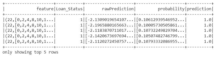
predictions = lr_model.transform(test_data)
predictions.show(5)The transform() method of the logistic regression model takes the test data as input and produces a new DataFrame predictions that includes the original columns from test_data along with additional columns, including the "prediction" column
Next we will create a metric for LogisticRegressionModel
predictions = lr_model.transform(test_data)
auc = BinaryClassificationEvaluator().setLabelCol('Loan_Status')
print('AUC:', str(auc.evaluate(predictions)))
We will apply the logistic regression model (lr_model) to the test data to generate predictions. The resulting DataFrame predictions contains the original columns from test_data along with additional columns, including the "prediction" column that contains the predicted class labels
The code BinaryClassificationEvaluator().setLabelCol('Loan_Status') creates an instance of the BinaryClassificationEvaluator and sets the label column to 'Loan_Status'. The BinaryClassificationEvaluator is used to evaluate the performance of binary classification models, such as logistic regression, by computing evaluation metrics like AUC-ROC
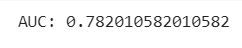
We got around 78% accuracy using LogisticRegressionModel
Next let us train the RandomForestClassifier model
rf = RandomForestClassifier(featuresCol='feature', labelCol='Loan_Status')
rf_model = rf.fit(train_data)
This creates an instance of the RandomForestClassifier in PySpark. The RandomForestClassifier is an ensemble classifier that fits multiple decision trees on different sub-samples of the dataset and averages the predictions to make the final classification
The arguments featuresCol and labelCol specify the names of the columns in the DataFrame that contain the features and the target variable, respectively
After creating the RandomForestClassifier instance, the code rf_model = rf.fit(train_data) fits the random forest model to the training data. The fit() method is called on the RandomForestClassifier object, and it trains the model using the features and target variable from the specified DataFrame
Next let us see the metric for RandomForestClassifier model
predictions = rf_model.transform(test_data)
auc = BinaryClassificationEvaluator().setLabelCol('Loan_Status')
print('AUC:', str(auc.evaluate(predictions)))
The code applies the trained random forest model (rf_model) to the test data (test_data) to make predictions. The transform() method of the random forest model takes the test data as input and produces a new DataFrame predictions that includes the original columns from test_data along with additional columns, including the "prediction" column
The BinaryClassificationEvaluator is used to evaluate the performance of binary classification models, such as random forest, by computing evaluation metrics like AUC-ROC
The evaluate() method computes the area under the ROC curve (AUC-ROC) based on the "prediction" column and the specified label column ('Loan_Status' in this case). The AUC value represents the performance of the random forest model in distinguishing between the two classes
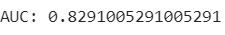
We got around 80% accuracy using RandomForestClassifier
Final Thoughts
PySpark provides a powerful and scalable framework for performing machine learning tasks
With PySpark's MLlib library, you can build and train machine learning models on large-scale datasets using distributed computing capabilities
Overall, PySpark simplifies the process of building and deploying machine learning models on large datasets by leveraging distributed computing capabilities. It allows you to harness the power of Apache Spark for efficient data processing and modeling, making it a valuable tool for big data analytics and machine learning tasks
In this project tutorial we have seen how we can create a Machine Learning model that can accurately predict loan approvals based on various features and also explored Logistic Regression and Random Forest algorithms. This project can also be extended by exploring different Machine Learning algorithms and improving the accuracy of the model
Get the project notebook from here
Thanks for reading the article!!!
Check out more project videos from the YouTube channel Hackers Realm


Comments