
Anime Face Generation using DCGAN | Keras Tensor flow | Deep Learning | Python
- Hackers Realm
- May 29, 2023
- 14 min read
Updated: May 31, 2023
Step into the world of anime face generation with Python! In this tutorial, explore the power of Deep Convolutional GANs (DCGAN) using Keras and TensorFlow. Unleash your creativity as you learn to generate high-quality anime faces from scratch. Dive into the realm of deep learning and enhance your skills in image generation and manipulation. Discover the fascinating intersection of technology and art with this comprehensive project tutorial. #AnimeFaceGeneration #DCGAN #Keras #TensorFlow #Python
Deep Convolutional Generative Adversarial Network (DCGAN) is a type of generative model that uses deep convolutional neural networks (CNNs) to generate new, realistic-looking images. DCGANs are a variation of the original GAN (Generative Adversarial Network) model, which consists of two neural networks: a generator and a discriminator.

In this project, we will see how we can generate new anime faces using DCGAN based on the training dataset. We will generate two models generator and discriminator. The generator network takes random noise as input and learns to generate synthetic images. The goal of the generator is to produce images that are indistinguishable from real images. The discriminator network, on the other hand, takes an image as input and learns to classify it as either real or generated. The discriminator's objective is to correctly classify real and generated images.
You can watch the video-based tutorial with a step-by-step explanation down below.
Dataset Information
The dataset for this project is downloaded from kaggle. The dataset consists of 21551 anime faces which are then cropped using the anime face detection algorithm. All images are resized to 64 * 64 for the sake of convenience
Import Modules
import os
import numpy as np
import matplotlib.pyplot as plt
import warnings
from tqdm.notebook import tqdm

import tensorflow as tf
from tensorflow import keras
from tensorflow.keras.preprocessing.image import load_img, array_to_img
from tensorflow.keras.models import Sequential, Model
from tensorflow.keras import layers
from tensorflow.keras.optimizers import Adam
from tensorflow.keras.losses import BinaryCrossentropy

warnings.filterwarnings('ignore')
os - used to handle files using system commands
numpy - used to perform a wide variety of mathematical operations on arrays
matplotlib - used for data visualization and graphical plotting
warnings - used to control and suppress warning messages that may be generated by the Python interpreter or third-party libraries during the execution of a Python program
tqdm.notebook - used for adding progress bars to your code in Jupyter Notebook
tensorflow - used for various tasks in machine learning and deep learning
tensorflow.keras.preprocessing.image - provides a variety of image preprocessing utilities for working with images in TensorFlow
tensorflow.keras.models - provides various classes and functions for creating and working with neural network models using the Keras API within TensorFlow
tensorflow.keras - provides an interface to build, train, and deploy deep learning models using the Keras API within TensorFlow
tensorflow.keras.optimizers - provides a collection of optimization algorithms that can be used to train deep learning models in TensorFlow using the Keras API
tensorflow.keras.losses - provides a collection of loss functions that can be used to measure the discrepancy between the predicted and target values during the training of deep learning models using the Keras API within TensorFlow
Load the Dataset
First we will create the base directory
BASE_DIR = '/kaggle/input/anime-faces/data/'Next we will create a list which will contain all the dataset images
# load complete image paths to the list
image_paths = []
for image_name in os.listdir(BASE_DIR):
    image_path = os.path.join(BASE_DIR, image_name)
    image_paths.append(image_path)
os.listdir() function retrieves a list of all files and directories present in the BASE_DIR directory
os.path.join() creates the complete path of the image file by joining the base directory path with the image name
The resulting image path is then appended to the image_paths list
Now let us see the image paths that has been generated
image_paths[:5]This will display the complete path of first 5 images
['/kaggle/input/anime-faces/data/21130.png', '/kaggle/input/anime-faces/data/9273.png', '/kaggle/input/anime-faces/data/18966.png', '/kaggle/input/anime-faces/data/14127.png', '/kaggle/input/anime-faces/data/18054.png']
There is some unnecessary file in the dataset , we will have to remove it
# remove unnecessary file
image_paths.remove('/kaggle/input/anime-faces/data/data')
remove() function is used to delete a file or a single item from a list
Next we will get length of image paths list
len(image_paths)21551
There 21551 image paths in the list as there are 21551 images in the dataset which we have provided
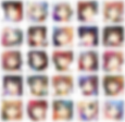
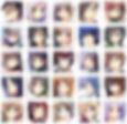
Visualize the Image Dataset
Next we will visualize few images in the dataset
# to display grid of images (7x7)
plt.figure(figsize=(20, 20))
temp_images = image_paths[:49]
index = 1

for image_path in temp_images:
    plt.subplot(7, 7, index)
    # load the image
    img = load_img(image_path)
    # convert to numpy array
    img = np.array(img)
    # show the image
    plt.imshow(img)
    plt.axis('off')
    # increment the index for next image
    index += 1
plt.figure(figsize=(20, 20)) creates a figure with a size of 20x20 inches
temp_images variable contains a subset of image paths . In this case the first 49 images
For each image in temp_images, set the subplot using plt.subplot() to position the current image in the 7x7 grid
Next load the image using load_img()
Convert the image to a NumPy array using np.array()
plt.imshow() displays the image
We don't want to show the axis labels, plt.axis('off') turns off the axis labels

Preprocess the Image Dataset
Next we will preprocess the dataset
# load the image and convert to numpy array
train_images = [np.array(load_img(path)) for path in tqdm(image_paths)]
train_images = np.array(train_images)
We will iterate over each image path in image_paths using list comprehension
For each path, the load_img() function is called to load the image as a PIL image object
Then, np.array() converts the PIL image object to a NumPy array. The resulting NumPy array is appended to the train_images list
The tqdm() function is used to wrap the iterable image_paths to display a progress bar during the iteration
After the list comprehension, the train_images list is converted to a NumPy array using np.array()
Next we will see the shape of the image
train_images[0].shape(64, 64, 3)
(64, 64, 3) is the dimensions of the image , the first two dimensions represent the spatial dimensions (height and width), and the last dimension represents the number of channels
Next we will reshape the numpy array
# reshape the array
train_images = train_images.reshape(train_images.shape[0], 64, 64, 3).astype('float32')
reshape() function is used to change the shape of the train_images array
This reshaping allows the images to be organized in a 4-dimensional array, where each image is represented as a 3D tensor
astype('float32') method is called on the train_images array. This converts the data type of the array elements to 'float32'
Next we will normalize the image
# normalize the images
train_images = (train_images - 127.5) / 127.5
Normalizes the array by scaling the pixel values to the range of [-1, 1]
the train_images array is subtracted by 127.5 and then divided by 127.5. This operation centers the pixel values around 0 and scales them to the range of [-1, 1]
Next let us see the preprocessed image
train_images[0]You will see the following result :
array([[[-0.7254902 , -0.90588236, -0.7176471 ],
[-0.70980394, -0.88235295, -0.6862745 ],
[-0.7019608 , -1. , -0.7176471 ],
...,
[-0.09019608, 0.01176471, 0.3882353 ],
[-0.19215687, 0.05882353, 0.4509804 ],
[-0.34117648, -0.13725491, 0.29411766]],
[[-0.7254902 , -0.90588236, -0.7176471 ],
[-0.73333335, -0.8666667 , -0.7019608 ],
[-0.52156866, -0.8666667 , -0.5686275 ],
...,
[-0.29411766, 0.01176471, 0.3019608 ],
[-0.08235294, 0.15294118, 0.5294118 ],
[-0.23921569, 0.09019608, 0.45882353]],
[[-0.7019608 , -0.8901961 , -0.7019608 ],
[-0.7176471 , -0.8745098 , -0.69411767],
[-0.5686275 , -0.8509804 , -0.58431375],
...,
[-0.22352941, 0.1764706 , 0.48235294],
[-0.13725491, 0.1764706 , 0.4745098 ],
[-0.06666667, 0.24705882, 0.5058824 ]],
...,
[[-0.30980393, -0.6862745 , -0.29411766],
[-0.34901962, -0.6862745 , -0.37254903],
[-0.30980393, -0.5372549 , -0.35686275],
...,
[-0.79607844, -0.9843137 , -0.77254903],
[-0.827451 , -0.8745098 , -0.85882354],
[-0.7647059 , -0.92156863, -0.8039216 ]],
[[-0.3254902 , -0.6392157 , -0.29411766],
[-0.44313726, -0.7254902 , -0.43529412],
[-0.54509807, -0.7882353 , -0.54509807],
...,
[-0.8352941 , -0.9764706 , -0.70980394],
[-0.7254902 , -0.8745098 , -0.75686276],
[-0.7411765 , -0.9137255 , -0.69411767]],
[[-0.5764706 , -0.827451 , -0.54509807],
[-0.56078434, -0.8666667 , -0.5294118 ],
[-0.58431375, -0.85882354, -0.5764706 ],
...,
[-0.7411765 , -0.8666667 , -0.6156863 ],
[-0.7254902 , -0.9372549 , -0.70980394],
[-0.7647059 , -0.92941177, -0.7176471 ]]], dtype=float32)
Create Generator & Discriminator Models
First we will initialize the required values to the variables
# latent dimension for random noise
LATENT_DIM = 100
# weight initializer
WEIGHT_INIT = keras.initializers.RandomNormal(mean=0.0, stddev=0.02)
# no. of channels of the image
CHANNELS = 3 # for gray scale, keep it as 1
LATENT_DIM variable represents the dimensionality of the random noise vector used as input for a generative model, such as a generative adversarial network (GAN) or a variational autoencoder (VAE)
The WEIGHT_INIT variable represents the weight initializer used to initialize the weights of the neural network model. In this case, it is set to a random normal initializer with a mean of 0.0 and a standard deviation of 0.02
The CHANNELS variable represents the number of channels in the image data. In this case, it is set to 3, indicating that the images are in RGB color format
Generator Model
Generator Model will create new images similar to training data from random noise
model = Sequential(name='generator')

# 1d random noise
model.add(layers.Dense(8 * 8 * 512, input_dim=LATENT_DIM))
model.add(layers.ReLU())

# convert 1d to 3d
model.add(layers.Reshape((8, 8, 512)))

# upsample to 16x16
model.add(layers.Conv2DTranspose(256, (4, 4), strides=(2, 2), padding='same', kernel_initializer=WEIGHT_INIT))
model.add(layers.ReLU())

# upsample to 32x32
model.add(layers.Conv2DTranspose(128, (4, 4), strides=(2, 2), padding='same', kernel_initializer=WEIGHT_INIT))
model.add(layers.ReLU())

# upsample to 64x64
model.add(layers.Conv2DTranspose(64, (4, 4), strides=(2, 2), padding='same', kernel_initializer=WEIGHT_INIT))
model.add(layers.ReLU())

model.add(layers.Conv2D(CHANNELS, (4, 4), padding='same', activation='tanh'))

generator = model
generator.summary()
The Sequential model is initialized with the name "generator"
The model starts with a Dense layer that takes 1D random noise as input. The number of units in this layer is 8 * 8 * 512, resulting in a 1D tensor with a length of 32768. The input_dim is set to the value of LATENT_DIM . This layer is followed by a ReLU activation function
The next layer is a Reshape layer that converts the 1D tensor into a 3D tensor with a shape of (8, 8, 512)
The model then uses a Conv2DTranspose layer to upsample the tensor to a size of 16x16. It uses 256 filters with a kernel size of (4, 4), strides of (2, 2), and "same" padding. The weights of this layer are initialized using the WEIGHT_INIT initializer. The output of this layer goes through a ReLU activation function
Another Conv2DTranspose layer is added to further upsample the tensor to a size of 32x32. This layer uses 128 filters with the same configuration as the previous layer. The output is again passed through a ReLU activation function.
The next Conv2DTranspose layer upsamples the tensor to a size of 64x64 using 64 filters and the same configuration as the previous layers. The output is then passed through a ReLU activation function.
Finally, a Conv2D layer with CHANNELS filters and a kernel size of (4, 4) is used to generate the output image. The activation function for this layer is set to "tanh", which scales the output between -1 and 1, representing the pixel intensities
This is the summary of the model's architecture is printed using the summary() method
Discriminator Model
Discriminator model will classify the image from the generator to check whether it real (or) fake images
model = Sequential(name='discriminator')
input_shape = (64, 64, 3)
alpha = 0.2

# create conv layers
model.add(layers.Conv2D(64, (4, 4), strides=(2, 2), padding='same', input_shape=input_shape))
model.add(layers.BatchNormalization())
model.add(layers.LeakyReLU(alpha=alpha))

model.add(layers.Conv2D(128, (4, 4), strides=(2, 2), padding='same', input_shape=input_shape))
model.add(layers.BatchNormalization())
model.add(layers.LeakyReLU(alpha=alpha))

model.add(layers.Conv2D(128, (4, 4), strides=(2, 2), padding='same', input_shape=input_shape))
model.add(layers.BatchNormalization())
model.add(layers.LeakyReLU(alpha=alpha))

model.add(layers.Flatten())
model.add(layers.Dropout(0.3))

# output class
model.add(layers.Dense(1, activation='sigmoid'))

discriminator = model
discriminator.summary()
The Sequential model is initialized with the name "discriminator".
The model starts with a Conv2D layer with 64 filters, a kernel size of (4, 4), and strides of (2, 2). The input shape of the layer is set to (64, 64, 3) to match the shape of the input images. The layer applies same padding to maintain the spatial dimensions.
A BatchNormalization layer is added after the first convolutional layer. Batch normalization helps normalize the activations and improve the training stability.
The output of the batch normalization layer is passed through a LeakyReLU activation function with a negative slope parameter (alpha) set to 0.2. LeakyReLU helps alleviate the issue of dead neurons and introduces some non-linearity.
Two more sets of Conv2D, BatchNormalization, and LeakyReLU layers are added. The second set has 128 filters, and the third set also has 128 filters. All layers in these sets use the same kernel size, strides, padding, and input shape as the first layer.
Following the convolutional layers, a Flatten layer is added to convert the 2D feature maps into a 1D tensor
A Dropout layer with a dropout rate of 0.3 is applied to reduce overfitting by randomly dropping a fraction of the connections during training.
Finally, a Dense layer with a single unit and a sigmoid activation function is added. This layer outputs a probability indicating the likelihood that the input image is real (as opposed to fake)
The resulting discriminator model is stored in the discriminator variable, and a summary of the model's architecture is printed using the summary() method
Create DCGAN
This is the important step of this project where we will combine both generator and discriminator model . We will train both the models at same time and update the weights with customized loss functions
class DCGAN(keras.Model):
    def __init__(self, generator, discriminator, latent_dim):
        super().__init__()
        self.generator = generator
        self.discriminator = discriminator
        self.latent_dim = latent_dim
        self.g_loss_metric = keras.metrics.Mean(name='g_loss')
        self.d_loss_metric = keras.metrics.Mean(name='d_loss')

    @property
    def metrics(self):
        return [self.g_loss_metric, self.d_loss_metric]

    def compile(self, g_optimizer, d_optimizer, loss_fn):
        super(DCGAN, self).compile()
        self.g_optimizer = g_optimizer
        self.d_optimizer = d_optimizer
        self.loss_fn = loss_fn

    def train_step(self, real_images):
        # get batch size from the data
        batch_size = tf.shape(real_images)[0]
        # generate random noise
        random_noise = tf.random.normal(shape=(batch_size, self.latent_dim))

        # train the discriminator with real (1) and fake (0) images
        with tf.GradientTape() as tape:
            # compute loss on real images
            pred_real = self.discriminator(real_images, training=True)
            # generate real image labels
            real_labels = tf.ones((batch_size, 1))
            # label smoothing
            real_labels += 0.05 * tf.random.uniform(tf.shape(real_labels))
            d_loss_real = self.loss_fn(real_labels, pred_real)

            # compute loss on fake images
            fake_images = self.generator(random_noise)
            pred_fake = self.discriminator(fake_images, training=True)
            # generate fake labels
            fake_labels = tf.zeros((batch_size, 1))
            d_loss_fake = self.loss_fn(fake_labels, pred_fake)

            # total discriminator loss
            d_loss = (d_loss_real + d_loss_fake) / 2

        # compute discriminator gradients
        gradients = tape.gradient(d_loss, self.discriminator.trainable_variables)
        # update the gradients
        self.d_optimizer.apply_gradients(zip(gradients, self.discriminator.trainable_variables))


        # train the generator model
        labels = tf.ones((batch_size, 1))
        # generator want discriminator to think that fake images are real
        with tf.GradientTape() as tape:
            # generate fake images from generator
            fake_images = self.generator(random_noise, training=True)
            # classify images as real or fake
            pred_fake = self.discriminator(fake_images, training=True)
            # compute loss
            g_loss = self.loss_fn(labels, pred_fake)

        # compute gradients
        gradients = tape.gradient(g_loss, self.generator.trainable_variables)
        # update the gradients
        self.g_optimizer.apply_gradients(zip(gradients, self.generator.trainable_variables))

        # update states for both models
        self.d_loss_metric.update_state(d_loss)
        self.g_loss_metric.update_state(g_loss)

        return {'d_loss': self.d_loss_metric.result(), 'g_loss': self.g_loss_metric.result()}
The above code snippet represents a DCGAN model implemented as a custom Keras model using the keras.Model subclass
The DCGAN class inherits from keras.Model
The __init__ method initializes the generator, discriminator, and latent dimension. It also sets up loss metrics for the generator and discriminator
The metrics property returns a list of metrics to be tracked during training. In this case, it includes the generator loss and discriminator loss metrics
The compile method is overridden to set the optimizers and loss function for training.
The train_step method defines a single training step for the DCGAN model.
Inside the training step, real images are passed as input.
Random noise is generated using tf.random.normal with the shape (batch_size, latent_dim)
The discriminator is trained first. A gradient tape is used to record the operations for differentiation.
The loss is computed for the real images by passing them through the discriminator. Label smoothing is applied to the real labels to improve training stability. The loss is calculated using the specified loss function
Then loss is computed for the fake images generated by the generator. The loss is calculated using the specified loss function and fake labels. The fake images are obtained by passing the random noise through the generator.
The total discriminator loss is computed as the average of the losses on real and fake images
Gradients of the discriminator loss with respect to the discriminator's trainable variables are computed using the tape.
The gradients are applied to the discriminator's trainable variables using the optimizer.
The generator is trained next. Another gradient tape is used to record the operations.
Fake labels are set to 1 because the generator aims to fool the discriminator into classifying fake images as real.
Fake images are generated by passing the random noise through the generator.
The fake images are passed through the discriminator, and the loss is computed using the specified loss function and fake labels.
Gradients of the generator loss with respect to the generator's trainable variables are computed using the tape.
The gradients are applied to the generator's trainable variables using the optimizer.
The loss metrics for both the generator and discriminator are updated.
The method returns a dictionary containing the discriminator loss and generator loss metrics
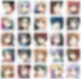
Next we will plot some images for each epoch
class DCGANMonitor(keras.callbacks.Callback):
    def __init__(self, num_imgs=25, latent_dim=100):
        self.num_imgs = num_imgs
        self.latent_dim = latent_dim
        # create random noise for generating images
        self.noise = tf.random.normal([25, latent_dim])

    def on_epoch_end(self, epoch, logs=None):
        # generate the image from noise
        g_img = self.model.generator(self.noise)
        # denormalize the image
        g_img = (g_img * 127.5) + 127.5
        g_img.numpy()

        fig = plt.figure(figsize=(8, 8))
        for i in range(self.num_imgs):
            plt.subplot(5, 5, i+1)
            img = array_to_img(g_img[i])
            plt.imshow(img)
            plt.axis('off')
        # plt.savefig('epoch_{:03d}.png'.format(epoch))
        plt.show()

    def on_train_end(self, logs=None):
        self.model.generator.save('generator.h5')
The DCGANMonitor class inherits from keras.callbacks.Callback
The __init__ method initializes the callback with the number of images to generate and the dimension of the latent space . It also creates a random noise tensor for generating images.
The on_epoch_end method is called at the end of each training epoch. Inside this method, the generator model is used to generate images by passing the random noise tensor through it.
The generated images are then denormalized by multiplying by 127.5 and adding 127.5 to bring the pixel values back to the range of [0, 255]
A figure is created using plt.figure, and a subplot grid is set up using plt.subplot
The generated images are plotted in the subplots using a loop. Each subplot represents one generated image
The array_to_img function is used to convert the image array into a PIL Image object, and plt.imshow is used to display the image.
The axis is turned off using plt.axis()
The plt.show() function is called to display the figure with the generated images.
The on_train_end method is called at the end of the training. It saves the generator model as a file named "generator.h5" using the save method
Now let us initialize the DCGAN model
dcgan = DCGAN(generator=generator, discriminator=discriminator, latent_dim=LATENT_DIM)The code snippet instantiates a DCGAN model using the provided generator, discriminator, and latent dimension
By passing the generator and discriminator models to the DCGAN constructor, you create a DCGAN model that consists of a generator and a discriminator working together in an adversarial manner
Next let us compile the DCGAN model
D_LR = 0.0001
G_LR = 0.0003
dcgan.compile(g_optimizer=Adam(learning_rate=G_LR, beta_1=0.5), d_optimizer=Adam(learning_rate=D_LR, beta_1=0.5), loss_fn=BinaryCrossentropy())
D_LR and G_LR defines the learning rates for discriminator and generator optimizer respectively
dcgan model is compiled using the compile method with g_optimizer in this case Adam optimizer is used with the specified learning rate and the momentum parameter beta_1 set to 0.5. The optimizer for the discriminator model in this case Adam optimizer is used with the specified learning rate and beta_1 set to 0.5. BinaryCrossentropy is used for loss function
By compiling the DCGAN model with the optimizers and loss function, the model is prepared for training
Next we will train the model
N_EPOCHS = 50
dcgan.fit(train_images, epochs=N_EPOCHS, callbacks=[DCGANMonitor()])
By calling the fit method, the DCGAN model starts training on the provided dataset. It will run for the specified number of epochs, and at the end of each epoch, the DCGANMonitor callback will generate and display the generated images. The training progress, including the discriminator and generator losses, will be displayed during the training process
You will see the following output
Epoch 1/50
674/674 [==============================] - 36s 41ms/step - d_loss: 0.6092 - g_loss: 2.7299
Epoch 2/50 674/674 [==============================] - 27s 41ms/step - d_loss: 0.5241 - g_loss: 1.9957
Epoch 3/50 674/674 [==============================] - 27s 41ms/step - d_loss: 0.5738 - g_loss: 1.8336

Epoch 10/50 674/674 [==============================] - 27s 40ms/step - d_loss: 0.6962 - g_loss: 1.0153
Epoch 20/50 674/674 [==============================] - 27s 41ms/step - d_loss: 0.7027 - g_loss: 0.7699
Epoch 30/50 674/674 [==============================] - 28s 41ms/step - d_loss: 0.6717 - g_loss: 0.8222
Epoch 40/50 674/674 [==============================] - 27s 40ms/step - d_loss: 0.6304 - g_loss: 0.9496
Epoch 50/50 674/674 [==============================] - 27s 40ms/step - d_loss: 0.5894 - g_loss: 1.0865
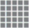
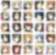
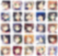
From the output we can see that first epoch has generated a image with some kind of noise
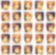
We can see that over each epoch the quality of images has improved
Generate New Anime Image
Next we will generate new image using trained dcgan model
noise = tf.random.normal([1, 100])
fig = plt.figure(figsize=(3, 3))
# generate the image from noise
g_img = dcgan.generator(noise)
# denormalize the image
g_img = (g_img * 127.5) + 127.5
g_img.numpy()
img = array_to_img(g_img[0])
plt.imshow(img)
plt.axis('off')
plt.show()
A random noise tensor is created with shape [1, 100] using tf.random.normal. This tensor represents the input to the generator model
A figure with a size of 3x3 is created using plt.figure
The generator model (dcgan.generator) is used to generate an image by passing the random noise tensor through it. The resulting tensor is stored in g_img
The generated image is denormalized by multiplying by 127.5 and adding 127.5 to bring the pixel values back to the range of [0, 255]
The numpy method is called on the g_img tensor to convert it to a NumPy array
The array_to_img function is used to convert the image array into a PIL Image object
The generated image is displayed using plt.imshow
The axis is turned off using plt.axis()
The plt.show() function is called to display the image

Final Thoughts
DCGANs have shown impressive results in generating realistic images across various domains, such as faces, objects, and scenes. They have been widely used in computer vision research and applications, including image synthesis, data augmentation, and image-to-image translation
It's important to note that while DCGANs can generate visually appealing images, they don't possess an understanding of the semantic meaning behind the images they generate
They learn statistical patterns from the training data and generate new samples based on those patterns
In this project tutorial, we have explored how DCGAN can be used to generate new anime faces . In future projects we can see how different GAN's can be used for generating new anime face images
Get the project notebook from here
Thanks for reading the article!!!
Check out more project videos from the YouTube channel Hackers Realm