
Dogs vs Cats Image Classification using Python | CNN | Deep Learning Project Tutorial
- Hackers Realm
- May 3, 2022
- 6 min read

Updated: May 15, 2024
Embark on the journey of image classification with Python! This tutorial explores CNN and deep learning techniques to classify images of dogs and cats. Learn to build accurate models that can distinguish between these furry friends, unlocking applications in pet recognition, animal monitoring, and more. Enhance your skills in computer vision, deep learning, and unleash the power of image classification. Join this comprehensive project tutorial to unravel the world of dogs vs cats image classification with python. #DogsVsCats #Python #CNN #DeepLearning #ImageClassification #ComputerVision

In this project tutorial we will use Convolutional Neural Network (CNN) for image feature extraction and visualize the results with plot graphs.
You can watch the video-based tutorial with step by step explanation down below.
Dataset Information
The training archive contains 25,000 images of dogs and cats. Train your algorithm on these files and predict the labels
(1 = dog, 0 = cat).
Download the dataset here
Environment: Google Colab
Download Dataset
We can download the dataset directly from the Microsoft page
!wget https://download.microsoft.com/download/3/E/1/3E1C3F21-ECDB-4869-8368-6DEBA77B919F/kagglecatsanddogs_3367a.zipa--2021-05-06 16:04:20-- https://download.microsoft.com/download/3/E/1/3E1C3F21-ECDB-4869-8368-6DEBA77B919F/kagglecatsanddogs_3367a.zip Resolving download.microsoft.com (download.microsoft.com)... 23.78.216.154, 2600:1417:8000:980::e59, 2600:1417:8000:9b2::e59 Connecting to download.microsoft.com (download.microsoft.com)|23.78.216.154|:443... connected. HTTP request sent, awaiting response... 200 OK Length: 824894548 (787M) [application/octet-stream] Saving to: ‘kagglecatsanddogs_3367a.zip’ kagglecatsanddogs_3 100%[===================>] 786.68M 187MB/s in 4.3s 2021-05-06 16:04:24 (183 MB/s) - ‘kagglecatsanddogs_3367a.zip’ saved [824894548/824894548]
Unzip the Dataset
!unzip kagglecatsanddogs_3367a.zipRun this code once and comment it
Import Modules
import pandas as pd
import numpy as np
import matplotlib.pyplot as plt
import warnings
import os
import tqdm
import random
from keras.preprocessing.image import load_img
warnings.filterwarnings('ignore')
pandas - used to perform data manipulation and analysis
numpy - used to perform a wide variety of mathematical operations on arrays
matplotlib - used for data visualization and graphical plotting
os - used to handle files using system commands
tqdm - progress bar decorator for iterators
random - used for randomizing
load_img - used for loading the image as numpy array
warnings - to manipulate warnings details, filterwarnings('ignore') is to ignore the warnings thrown by the modules (gives clean results)
Create Dataframe for Input and Output
The Dogs vs Cats dataset may differ from where it was downloaded like folder structures or labels. You may create a dataframe to convert the input and output paths accordingly for easier processing.
input_path = []
label = []

for class_name in os.listdir("PetImages"):
    for path in os.listdir("PetImages/"+class_name):
        if class_name == 'Cat':
            label.append(0)
        else:
            label.append(1)
        input_path.append(os.path.join("PetImages", class_name, path))
print(input_path[0], label[0])
PetImages/Dog/4253.jpg 1
Adding the label to the images, one (1) for dogs and zero (0) for cats
Display the path of first image with corresponding label
Now we create the dataframe for processing
df = pd.DataFrame()
df['images'] = input_path
df['label'] = label
df = df.sample(frac=1).reset_index(drop=True)
df.head()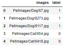
Display of image paths with labels
Data was shuffled and the index was removed
We must remove any files in the data set that are not image data to avoid errors
for i in df['images']:
    if '.jpg' not in i:
        print(i)
PetImages/Cat/Thumbs.db PetImages/Dog/Thumbs.db
import PIL
l = []
for image in df['images']:
    try:
        img = PIL.Image.open(image)
    except:
        l.append(image)
l
['PetImages/Cat/666.jpg', 'PetImages/Cat/Thumbs.db', 'PetImages/Dog/Thumbs.db', 'PetImages/Dog/11702.jpg']
List of non-image type files and corrupted images
# delete db files
df = df[df['images']!='PetImages/Dog/Thumbs.db']
df = df[df['images']!='PetImages/Cat/Thumbs.db']
df = df[df['images']!='PetImages/Cat/666.jpg']
df = df[df['images']!='PetImages/Dog/11702.jpg']
len(df)
24998
Dropping the corrupted files and non-image files from the dataset
Exploratory Data Analysis
Let us display a grid of images to know the content of the data
# to display grid of images
plt.figure(figsize=(25,25))
temp = df[df['label']==1]['images']
start = random.randint(0, len(temp))
files = temp[start:start+25]

for index, file in enumerate(files):
    plt.subplot(5,5, index+1)
    img = load_img(file)
    img = np.array(img)
    plt.imshow(img)
    plt.title('Dogs')
    plt.axis('off')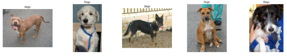
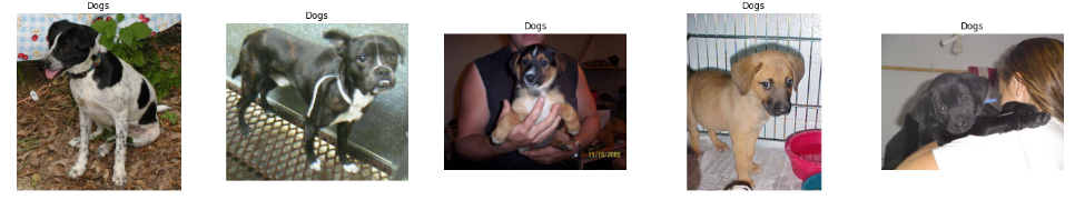
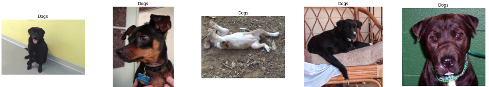
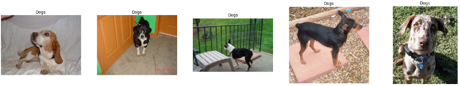
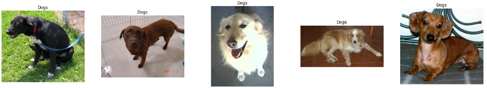
Display of 25 random images of dogs
plt.axis('off') turns off both axis from the images
Files loaded and stored in an array
# to display grid of images
plt.figure(figsize=(25,25))
temp = df[df['label']==0]['images']
start = random.randint(0, len(temp))
files = temp[start:start+25]

for index, file in enumerate(files):
    plt.subplot(5,5, index+1)
    img = load_img(file)
    img = np.array(img)
    plt.imshow(img)
    plt.title('Cats')
    plt.axis('off')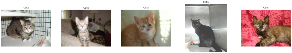
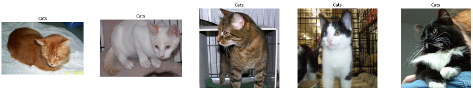
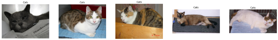
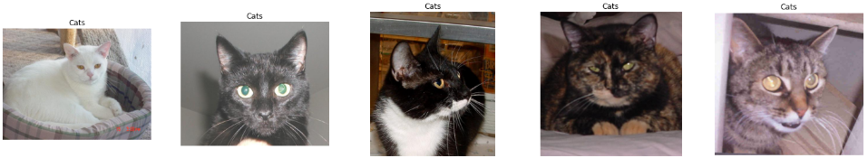
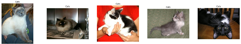
Display of 25 random images of cats
Different saturation and qualities among the images
import seaborn as sns
sns.countplot(df['label'])
seaborn - built on top of matplotlib with similar functionalities
We can observe an equal distribution of both classes
Create Data Generator for the Images
Data Generators loads the data from the disk for reading and training the data directly, saving RAM space and avoiding possible overflow that might crash the system.
df['label'] = df['label'].astype('str')
df.head()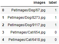
Convert the data type of 'label' to string for easier processing
Let us split the input data
# input split
from sklearn.model_selection import train_test_split
train, test = train_test_split(df, test_size=0.2, random_state=42)
from keras.preprocessing.image import ImageDataGenerator
train_generator = ImageDataGenerator(
rescale = 1./255, # normalization of images
rotation_range = 40, # augmention of images to avoid overfitting
shear_range = 0.2,
zoom_range = 0.2,
horizontal_flip = True,
fill_mode = 'nearest'
)
val_generator = ImageDataGenerator(rescale = 1./255)
train_iterator = train_generator.flow_from_dataframe(
train,x_col='images',
y_col='label',
target_size=(128,128),
batch_size=512,
class_mode='binary'
)
val_iterator = val_generator.flow_from_dataframe(
test,x_col='images',
y_col='label',
target_size=(128,128),
batch_size=512,
class_mode='binary'
)Found 19998 validated image filenames belonging to 2 classes. Found 5000 validated image filenames belonging to 2 classes.
Image Generator rescale and normalizes the images by pixels between 0 and 1 for easier processing.
Augmentation applied to transform the images for more angles
batch_size=512 - amount of images to process per iteration
Assign batch size according to the hardware specs
class_mode='binary' indicates that there are 2 types of classes
Model Creation
from keras import Sequential
from keras.layers import Conv2D, MaxPool2D, Flatten, Dense

model = Sequential([
            Conv2D(16, (3,3), activation='relu', input_shape=(128,128,3)),
            MaxPool2D((2,2)),
            Conv2D(32, (3,3), activation='relu'),
            MaxPool2D((2,2)),
            Conv2D(64, (3,3), activation='relu'),
            MaxPool2D((2,2)),
            Flatten(),
            Dense(512, activation='relu'),
            Dense(1, activation='sigmoid')
])
Dense - single dimension linear layer array
Conv2D - convolutional layer in 2 dimension
MaxPooling2D - function to get the maximum pixel value to the next layer
Flatten - convert 2D array into a 1D array
Use Dropout if augmentation was not applied on the images to avoid over fitting
activation='relu' - used commonly for image classification models
input_shape=(128,128,3) - Resolution size of the images in an RGB color scales. If in grayscale the third parameter is 1.
activation='sigmoid' - used for binary classification
model.compile(optimizer='adam', loss='binary_crossentropy', metrics=['accuracy'])
model.summary()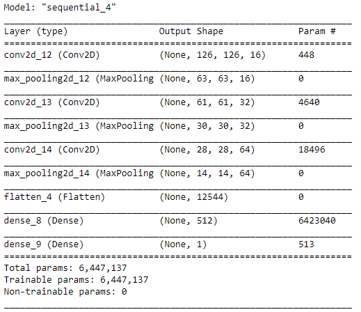
model.compile() - compilation of the model
optimizer=’adam’ - automatically adjust the learning rate for the model over the no. of epochs
loss='binary_crossentropy' - loss function for binary outputs
history = model.fit(train_iterator, epochs=10, validation_data=val_iterator)Epoch 1/10 40/40 [==============================] - 150s 4s/step - loss: 0.8679 - accuracy: 0.5187 - val_loss: 0.6399 - val_accuracy: 0.6238 Epoch 2/10 40/40 [==============================] - 147s 4s/step - loss: 0.6280 - accuracy: 0.6416 - val_loss: 0.5672 - val_accuracy: 0.7024 Epoch 3/10 40/40 [==============================] - 146s 4s/step - loss: 0.5737 - accuracy: 0.6980 - val_loss: 0.5493 - val_accuracy: 0.7148 Epoch 4/10 40/40 [==============================] - 146s 4s/step - loss: 0.5478 - accuracy: 0.7221 - val_loss: 0.5351 - val_accuracy: 0.7356 Epoch 5/10 40/40 [==============================] - 145s 4s/step - loss: 0.5276 - accuracy: 0.7338 - val_loss: 0.5104 - val_accuracy: 0.7494 Epoch 6/10 40/40 [==============================] - 144s 4s/step - loss: 0.5127 - accuracy: 0.7405 - val_loss: 0.4853 - val_accuracy: 0.7664 Epoch 7/10 40/40 [==============================] - 144s 4s/step - loss: 0.5059 - accuracy: 0.7544 - val_loss: 0.4586 - val_accuracy: 0.7868 Epoch 8/10 40/40 [==============================] - 143s 4s/step - loss: 0.4842 - accuracy: 0.7644 - val_loss: 0.5054 - val_accuracy: 0.7510 Epoch 9/10 40/40 [==============================] - 143s 4s/step - loss: 0.4971 - accuracy: 0.7530 - val_loss: 0.4647 - val_accuracy: 0.7894 Epoch 10/10 40/40 [==============================] - 142s 4s/step - loss: 0.4642 - accuracy: 0.7770 - val_loss: 0.4711 - val_accuracy: 0.7782
Assign the no. of epochs and batch size according to the hardware specifications
Training accuracy and validation accuracy increases each iteration
Training loss and validation loss decreases each iteration
Visualization of Results
acc = history.history['accuracy']
val_acc = history.history['val_accuracy']
epochs = range(len(acc))
plt.plot(epochs, acc, 'b', label='Training Accuracy')
plt.plot(epochs, val_acc, 'r', label='Validation Accuracy')
plt.title('Accuracy Graph')
plt.legend()
plt.figure()
loss = history.history['loss']
val_loss = history.history['val_loss']
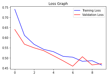
plt.plot(epochs, loss, 'b', label='Training Loss')
plt.plot(epochs, val_loss, 'r', label='Validation Loss')
plt.title('Loss Graph')
plt.legend()
plt.show()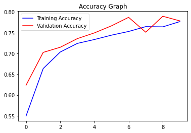
Highest training accuracy was 78.6
Highest validation accuracy was 78.9
Lowest training loss was 46.42
Lowest validation loss was 46.47
Test with Real Image
image_path = "test.jpg" # path of the image
img = load_img(image_path, target_size=(128, 128))
img = np.array(img)
img = img / 255.0 # normalize the image
img = img.reshape(1, 128, 128, 3) # reshape for prediction
pred = model.predict(img)
if pred[0] > 0.5:
    label = 'Dog'
else:
    label = 'Cat'
print(label)
'Dog'
Apply the same preprocessing step from the previous cells and predict the probability from the model
If the probability is greater than 0.5, the label will be 'Dog' and for probability less than 0.5, the label will be 'Cat'
You can adjust the probability threshold and analyze the performance difference
Final Thoughts
Training the model by increasing the no. of epochs can give better and more accurate results.
Processing large amount of data can take a lot of time and system resource.
Basic deep learning model trained in a small neural network, adding new layers varies the results.
You may use other image classification models of your preference for comparison.
In this project tutorial, we have explored the Dogs vs Cats dataset as a classification deep learning project. This is a basic deep learning project to learn image classification analysis and visualize the results through different plots.
Get the project notebook from here
Thanks for reading the article!!!
Check out more project videos from the YouTube channel Hackers Realm


Comments